Interpreting Experimental Results

PathPilot is an AI-powered internship matching platform. Think of it as a recommendation engine for early-career opportunities. Students fill out a profile that includes a proprietary personality and career motivation survey, and the algorithm surfaces internships tailored to their skills, interests, and unique preferences. The free tier gives you five matches a month. The premium subscription ($14.99/month) unlocks unlimited matches, resume optimization, and mock interview prep.

The company is preparing for a campus marketing blitz. Before they start spending scarce marketing dollars, they need to answer a simple question: which ad message is likely to drive more interest in the premium plan? They designed a randomized experiment. A sample of 240 college students were randomly assigned to see one of two ads for PathPilot Premium:

• “AI-Powered” (feature-focused): “PathPilot uses advanced AI to find your perfect internship match.”
• “3x Interviews” (outcome-focused): “PathPilot users land 3x more interviews than students who search on their own.”

After viewing the ad, each respondent answered: “How likely are you to subscribe to PathPilot Premium?” on a 1–5 scale, where 1 means “definitely would not subscribe” and 5 means “definitely would subscribe.”

The marketing team thinks the “3x interviews” is going to work best, but the CMO disagrees. He advised, ” if it don’t say AI, it ain’t going to fly.”

OK, Boomer!

This is why we do experiments.

In addition to the test data, the team will also collect some background information, such as whether the student is actively job searching and their year in school. Those variables will matter later. For now, we have one clean experimental question and one outcome. Let’s start there.

The Data

The dataset (pathpilot-experiment.csv) contains 240 respondents from a randomized online experiment. Each row is one participant.

Variable	Type	Description
response_id	ID	Unique respondent identifier
condition	Factor (2 levels)	Ad message shown: “AI-Powered” or “3x Interviews”
job_searching	Factor (Yes/No)	Whether the respondent is actively looking for an internship or job
year	Factor (4 levels)	Year in school: Freshman, Sophomore, Junior, or Senior
purchase_intent	Numeric (1–5)	Likelihood of subscribing to PathPilot Premium

Here’s a quick look at the two groups:

df |>
  group_by(condition) |>
  summarise(
    n = n(),
    mean_intent = mean(purchase_intent, na.rm = TRUE),
    sd = sd(purchase_intent, na.rm = TRUE)
  ) |>
  mutate(across(where(is.numeric), ~round(., 2))) |>
  gt() |>
  cols_label(
    condition = "Ad Condition",
    n = "N",
    mean_intent = "Mean Purchase Intent",
    sd = "SD"
  ) |>
  cols_align(columns = condition, align = "left") |>
  cols_width(
    condition ~ px(200),
    mean_intent ~ px(140),
    sd ~ px(80)
  )

Ad Condition	N	Mean Purchase Intent	SD
AI-Powered	120	3.12	0.88
3x Interviews	120	3.56	1.07

The averages look different. The outcome-focused message seems to be pulling ahead. But looking different isn’t enough. We need to know if the difference is real or if it could just be a fluke of who ended up in each group. This is exactly what a t-test is built for.

What a T-Test Does

A t-test answers the most basic question you usually want to answer when you do a marketing experiment: was our hunch (or hypothesis) right or not?

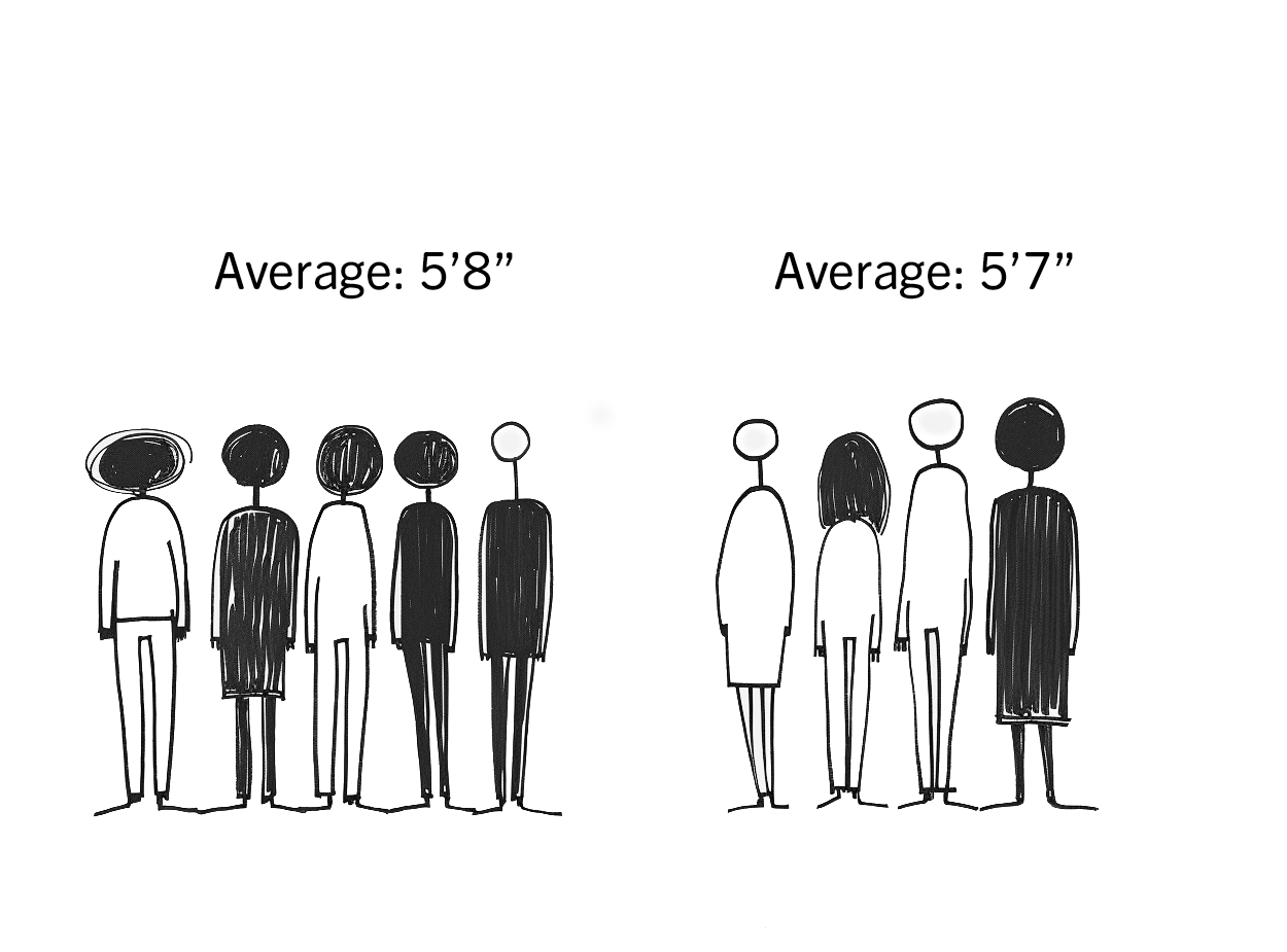
You have two groups. Each group saw a different ad. You measured the same outcome for both. The averages came back different. But averages are almost always a little different, even when nothing is going on. If you split 240 random people into two groups and measured their heights, the group averages would almost certainly be slightly different, just by chance. Doesn’t mean one group is actually taller.

The t-test tells you whether the gap between your two groups is big enough to be taken seriously, or whether it’s the kind of difference that could easily happen by luck alone.

The test looks at two things. First, how far apart are the group averages. Then, how much the individual scores within each group are bouncing around. If the averages are far apart and the scores within each group are fairly tight, we’re in good shape. The gap is probably worth our attention. If the averages are close together and individual scores are all over the place, the gap could easily be noise.

You can think of it as a ratio:

\[t = \frac{\text{How far apart are the group averages?}}{\text{How much are individual scores bouncing around?}}\]

When this ratio is big, it means the gap between groups is large compared to the messiness within them. When it’s small, the gap could easily be noise. The t-test then converts this ratio into a p-value—a single number that tells you how likely you’d be to see a gap this large if the ad actually made no difference at all.

It’s not magic. It’s just math. Fortunately, you don’t have to do it. That’s why we have computers.

In academia, if the p-value is below 0.05, we call the result statistically significant. That means there’s less than a 5% chance the difference is just random noise. Out “in the wild” (meaning in real companies), a p-value below 0.10 is often sufficient, meaning there’s less than a 10% chance what we’re seeing is random, luck-of-the-draw.

Interpreting the Results of a T-Test

Below, you can see the sample output of a T-Test. This one was done in R, but the output is similar to what you’d find in any software—even Excel.

library(broom)
library(gt)

t_result <- t.test(purchase_intent ~ condition, data = df)

t_result |> 
  tidy() |> 
  select(estimate1, estimate2, statistic, p.value) |> 
  gt() |>
  fmt_number(columns = where(is.numeric), decimals = 2) |>
  cols_label(
    estimate1 = "AI-Powered",
    estimate2 = "3x Interviews",
    statistic = "t",
    p.value = "p-value"
  ) |>
  tab_spanner(
    label = "Average Purchase Intent",
    columns = c(estimate1, estimate2)
  )

Average Purchase Intent		t	p-value
AI-Powered	3x Interviews
3.12	3.56	−3.44	0.00

Here’s how to decode:

What You See	What It Means
Average Purchase Intent	The average score for each group — the thing you’re actually comparing
t	The ratio we just talked about (Bigger numbers = stronger evidence)
p-value	Below the threshold (usually 0.05), the difference is real. Above it, you can’t be sure

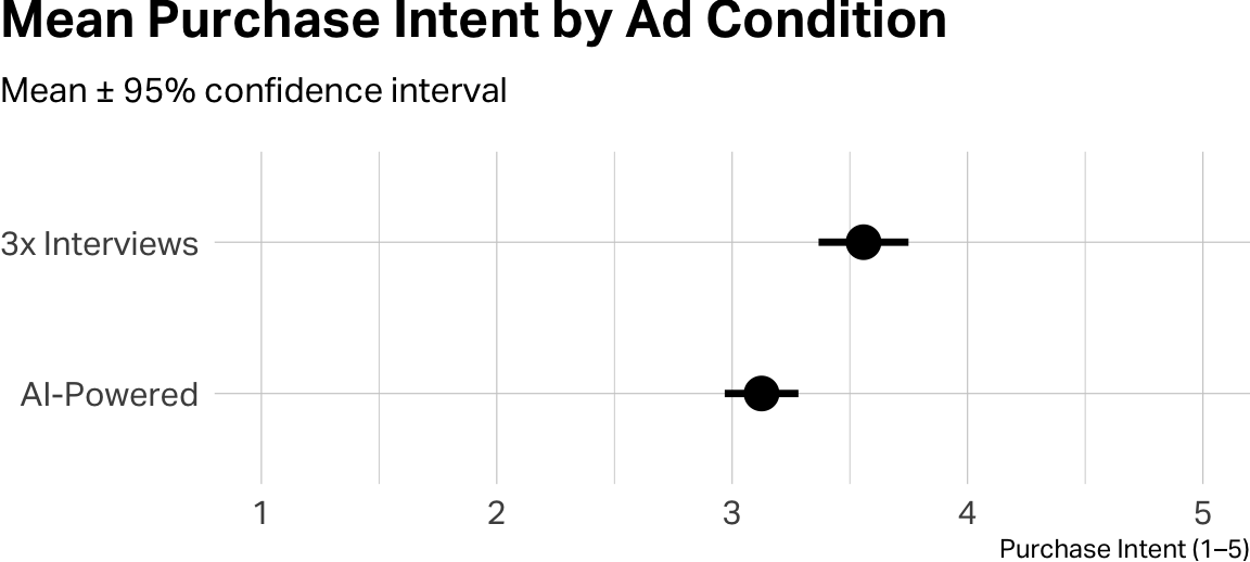
The “3x Interviews” group has an average purchase intent of 3.56, compared to 3.12 for the “AI-Powered” group. The p-value is 0.0007, about as good as it gets. That means this gap is almost certainly not a coincidence. The outcome-focused message genuinely drives higher interest.

If you were writing this up for PathPilot’s marketing team, you’d say something like, “The outcome-focused ad generated significantly higher purchase intent than the feature-focused ad.” The t-test is what lets you say “significantly” with confidence.

A quick visual makes the story easy to see:

df |>
  group_by(condition) |>
  summarise(
    mean_intent = mean(purchase_intent, na.rm = TRUE),
    se = sd(purchase_intent, na.rm = TRUE) / sqrt(n()),
    .groups = "drop"
  ) |>
  ggplot(aes(x = condition, y = mean_intent)) +
  geom_pointrange(
    aes(ymin = mean_intent - 1.96 * se, ymax = mean_intent + 1.96 * se),
    linewidth = 1.2,
    size = 1.1
  ) +
  coord_flip() +
  scale_y_continuous(limits = c(1, 5)) +
  labs(
    title = "Mean Purchase Intent by Ad Condition",
    subtitle = "Mean ± 95% confidence interval",
    x = NULL,
    y = "Purchase Intent (1–5)"
  ) +
  theme(plot.title.position = "plot")

The dots are the group averages. The horizontal lines show the range where the true average probably falls (remember, the average we are depicting is an estimate. The lines show the probable range that estimate could actually be. The important part is the relationship between the dots and the lines. When the ranges don’t overlap much, it’s a visual clue that the difference is probably real, which is exactly what the t-test just confirmed with the p-value.

What About More Than Two Groups?

The t-test is built for exactly two groups. But what if, at the last minute, PathPilot’s CMO had another idea to test. Say, he suggested a social proof message like, “Join 100,000 students already on PathPilot”. For this, a t-test won’t do the job. Here, we’d need ANOVA (short for ANalysis Of VAriance). It does the same kind of comparison, but it can handle three or more groups at once without getting tripped up. You may recall that we discussed this in a different teaching note.

The Limits of a Simple Comparison

So the t-test told us the “3x Interviews” message wins. Case closed?

Not quite.

The t-test told us that the groups scored differently. It didn’t tell us why. And it really only evaluated whether or not the outcomes were meaningfully different. It didn’t consider other influences that might have shaped the outcome. A senior staring down graduation is probably more interested in an internship tool than a freshman who just moved into their dorm, regardless of which ad they see. And a student who’s actively job searching is probably more motivated to subscribe than one who isn’t thinking about it yet. These factors could shape purchase intent, too. The t-test doesn’t consider them.

Think about it from PathPilot’s perspective. Knowing which ad to run is helpful. But knowing how well the ad worked independent of other influences would be really helpful. To get that fuller picture, we need a tool like linear regression, which lets you look at multiple factors at the same time and figure out how much each one matters.

If you want to see it as a formula (it’s ok if you don’t), it looks like this:

\[\text{Purchase Intent} = b_0 + b_1(\text{Ad Condition}) + b_2(\text{Job Searching}) + b_3(\text{Year}) + \text{noise}\]

The translation is simply this: a person’s purchase intent score is predicted by a combination of which ad they saw (\(b_1\)), whether they’re job searching (\(b_2\)), what year they’re in (\(b_3\)), plus some random individual stuff the model can’t explain (that’s the “noise,”which is usually referred to as error \(\epsilon\)). The \(b\) values are just numbers the model calculated to tell you how much each factor moves the needle. We’ll look at those numbers in a moment.

Running the Regression

Depending on the tool you’re using to build your regression model, the output can sometimes have more data than you need. What you really care about is the estimates for those calculated values (known as coefficients), the p-value for each, the p-value for the model, and a measure of how well the model fits the data, known simply as r-squared.

df <- df |> mutate(year_num = as.numeric(year))

model_reg <- lm(purchase_intent ~ condition + job_searching + year_num, data = df)

tidy(model_reg, conf.int = TRUE) |>
  mutate(
    term = case_when(
      term == "(Intercept)" ~ "Intercept (baseline)",
      term == "condition3x Interviews" ~ "Ad: 3x Interviews (vs. AI-Powered)",
      term == "job_searchingYes" ~ "Job Searching: Yes (vs. No)",
      term == "year_num" ~ "Year in School (1=Fr, 2=So, 3=Jr, 4=Sr)"
    )
  ) |>
  mutate(across(where(is.numeric), ~round(., 3))) |>
  gt() |>
  cols_label(
    term = "Predictor",
    estimate = "Coefficient",
    std.error = "SE",
    statistic = "t",
    p.value = "p-value",
    conf.low = "Lower CI",
    conf.high = "Upper CI"
  ) |>
  cols_align(align = "left", columns = term) |>
  cols_width(
    term ~ px(280),
    estimate ~ px(80),
    p.value ~ px(70)
  )

Predictor	Coefficient	SE	t	p-value	Lower CI	Upper CI
Intercept (baseline)	2.171	0.201	10.830	0.000	1.776	2.567
Ad: 3x Interviews (vs. AI-Powered)	0.449	0.116	3.866	0.000	0.220	0.678
Job Searching: Yes (vs. No)	0.734	0.122	6.018	0.000	0.494	0.974
Year in School (1=Fr, 2=So, 3=Jr, 4=Sr)	0.165	0.058	2.867	0.005	0.052	0.279

This table is the entire story. Well, almost. We also need the model fit statistics:

glance(model_reg) |>
  select(r.squared, statistic, p.value, nobs) |>
  gt() |>
  tab_header(title = "Model Fit Statistics") |> 
  fmt_number(columns = where(is.numeric), decimals = 3) |>
  cols_label(
    r.squared = "R²",
    statistic = "F",
    p.value = "p-value",
    nobs = "N"
  )

Model Fit Statistics
R²	F	p-value	N
0.200	19.658	0.000	240.000

Let’s walk through it all.

First, the columns — what each one means:

Column	Plain English
Coefficient	How much does this factor move the score? This is the main number you care about
SE	How precise is that estimate? Smaller is better
t	How confident should we be? Bigger numbers = more confident (same idea as the t-test)
p-value	Same rule as before — below 0.05 means this factor has a real effect
Lower CI / Upper CI	A range where the true effect probably falls. If this range doesn’t include zero, you’re in good shape

The rows are where the actual insights live:

The Intercept is the starting point. Every model has to start somewhere. The baseline is ours: for a Freshman who is not job searching and saw the “AI-Powered” ad, the predicted purchase intent is 2.17.

The Ad: 3x Interviews row tells you how much higher (or lower) the score is for people who saw the outcome-focused ad compared to people who saw the feature-focused ad. Crucially, this is the ad effect after the model has already accounted for whether someone is job searching and what year they’re in. Controlling for job search status and year in school, students who saw the “3x Interviews” ad scored 0.43 points higher on purchase intent than students who saw the “AI-Powered” ad.

The Job Searching row tells you how much higher (or lower) the score is for students who are actively looking for jobs compared to students who aren’t. Controlling for ad condition and year in school, students who are actively job searching scored 0.73 points higher on purchase intent than students who are not.

The Year in School row tells you the effect of each step up in class year (Freshman → Sophomore → Junior → Senior). Controlling for ad condition and job search status, each additional year in school is associated with 0.165 more points of purchase intent.

So what is this model actually telling us?

The ad still matters. Even after accounting for job search status and year, people who saw the “3x Interviews” ad scored 0.449 points higher on purchase intent (p = 10^{-4}). The message effect is real and it isn’t being explained away by the other factors.

Job searching matters (a lot). Students who are actively looking for a job or internship scored 0.734 points higher (p = 0), no matter which ad they saw. This is huge for PathPilot. It tells them something the t-test never could: who to target.

Year in school matters. Each additional year of school is associated with about 0.165 more points of purchase intent (p = 0.0045). Juniors and seniors are more interested than freshmen and sophomores. Not shocking, but now we have a number attached to it.

One last number worth knowing: the model’s R² is 0.2. In plain terms, that means these three factors together explain about 20% of what drives purchase intent. The other 80% is individual stuff we didn’t measure—personality, mood, whether someone’s roommate just got an amazing internship and now they’re motivated. An R² in this range is normal for survey data. You’re not trying to explain everything; you’re trying to find the factors that matter most.

What This Means in Practice

This is the real payoff. Look at the difference in what each tool told us:

• The t-test suggested PathPilot should probably run the outcome-focused ad. That’s a creative decision.

• The regression suggested PathPilot should probably run the outcome-focused ad because it still held the most sway even after we accounted for the influence of year in school and whether or not the student was actively job searching. That’s a solid pressure test.

Same data. Same experiment. But regression gave us a much richer set of answers because it looked at multiple factors at once instead of just two groups side by side.

Here’s a simple way to remember when to use each tool:

Tool	When to Use It	What It Tells You
T-Test	You tested two options and want to know which one won	Whether the two groups are really different or if it's just noise
ANOVA	You tested three or more options	Whether any of the groups differ, and which specific pairs are different
Linear Regression	You want to know the effect of your treatment while also understanding what other factors matter	The effect of each factor, cleaned of the influence of all the others

None of these tools is “better” than the others. They answer different questions. If you have two groups and just want to know if the treatment worked, a t-test is all you need. If you have three or more groups, use ANOVA. If you want to understand the treatment effect and figure out what other factors are at play, regression is the one.

In practice, most professional researchers will run a regression even when they only have two experimental conditions, because it lets them check whether other factors are influencing the result. The t-test is your starting point. Regression is where you go when you want the full picture.

A Few Cautions

A few things to keep in mind.

A “significant” result doesn’t automatically mean it’s important. If the “3x Interviews” ad only increased purchase intent by 0.05 points on a 5-point scale, nobody would care, even if the p-value was below 0.05. With a big enough sample, even tiny, meaningless differences can test as “significant.” Always look at the actual size of the difference, not just whether the p-value cleared the bar.

Regression doesn’t automatically prove cause and effect. In this study, we can reasonably infer that the ad caused the difference in purchase intent, because random assignment ensured the two groups were comparable before they saw anything. But we should be more careful about the other variables. The regression showed that job searching predicts higher intent. That’s not the same as saying job searching causes it. Something else might be going on. Maybe students who are job searching are also more motivated or more engaged with career tools in general. The ability to make a causal claim comes from how the experiment was designed, not from the math.

None of this works if the experiment was poorly designed. If the randomization was broken, if respondents could see both ads, or if your sample doesn’t represent the people you actually care about, no statistical test will fix it.

Further Reading

Field, A. (2024). Discovering Statistics Using R and RStudio (2nd ed.). SAGE. Chapters 10 (t-tests) and 13 (regression) are clear, practical, and written for humans, not robots.

Llaudet, E. & Imai, K. (2022). Data Analysis for Social Science: A Friendly and Practical Introduction. Princeton University Press. An excellent and accessible introduction to regression for students who haven’t taken a statistics course.