You’ve just closed your first survey. Eighty-seven people rated their satisfaction with a local coffee shop on a 1-to-5 scale. Your team is huddled around a laptop. Someone asks the obvious question: “So… what’s our number?”
Good question. What is your number?
Do you calculate the mean? “Average satisfaction: 3.8 out of 5.” Clean. Precise. Fits nicely on a slide.
Do you report the median? “The typical response was a 4.” Maybe more intuitive. Doesn’t get distorted by outliers.
Or do you skip the summary statistic entirely and just count the responses? “72% rated us a 4 or 5.” That’s the “top-two-box” score, and it’s what most brand trackers actually report.
All three are legitimate. All three will produce a different number from the same data. Unfortunately, the data doesn’t tell you which one to use. You have to decide.

This teaching note is a guide to making those decisions. It’s short on theory and long on practical advice. By the end, you should be able to open your survey results and know what to look for, what to calculate, and what questions to ask before you start making claims.
I: Before You Touch a Single Number
Ask an experienced researcher which statistic to calculate first and they’ll give you the same answer: don’t calculate anything. The first step is to take a look at your data.
| ID | Q1 | Q2 | Q3 | Q4 | Q5 | Duration | Open-End |
|---|---|---|---|---|---|---|---|
| 001 | 4 | 3 | 5 | 4 | 3 | 8:42 | “The staff was friendly but the wait was too long” |
| 002 | 3 | 3 | 3 | 3 | 3 | 2:14 | “good” |
| 003 | 5 | 4 | 4 | 5 | 4 | 9:17 | “I love coming here on weekends with my family” |
| 004 | 2 | 5 | 1 | 4 | 2 | 0:47 | “asdfasdf” |
| 005 | 4 | 4 | 5 | 3 | 4 | 7:53 | “Coffee is great, parking is terrible” |
You’re looking for obvious problems. Did someone answer every question with the same number (ID 002)? That’s a straight-liner—they might not have been paying attention. Did someone finish a 10-minute survey in 47 seconds (ID 004)? Did someone write “asdfasdf” in an open-ended response (ID 004)? Bot or bored human? Either way, garbage.
You’d be amazed how often students and junior analysts skip this step and end up building their entire analysis on polluted data. They calculate means, build charts, and write up findings on data that is tainted by 15% of responses that probably came from people who were watching TikTok while auto-clicking through their carefully designed survey.
Later in the course, we’ll cover statistical techniques that can identify bad respondents efficiently, and guidelines for when it may be appropriate to remove them. For now, build the habit of looking before you calculate.
Look first. Clean second. Analyze third.
II: The Building Blocks
Once your data is clean, you have a small toolkit of summary measures. Each one tells you something different. Here’s the cheat sheet:
| Measure | What It Tells You | When It Misleads |
|---|---|---|
| Counts | How many people said X | When you forget that n=6 isn’t a trend |
| Percentages | What share said X | When you ignore the base (35% of 20 ≠ 35% of 200) |
| Mean | The mathematical average | When the distribution is skewed or bimodal |
| Median | The midpoint response | When you care about what’s happening at the extremes—the median ignores them entirely |
| Standard Deviation | How much responses vary | When you report it without context (SD of what?) |
| Top-Two-Box | % who gave the highest responses | When you have a polarized distribution. A high T2B can hide a large group of detractors |
Let’s walk through each one.
Counts and Percentages: The Foundation
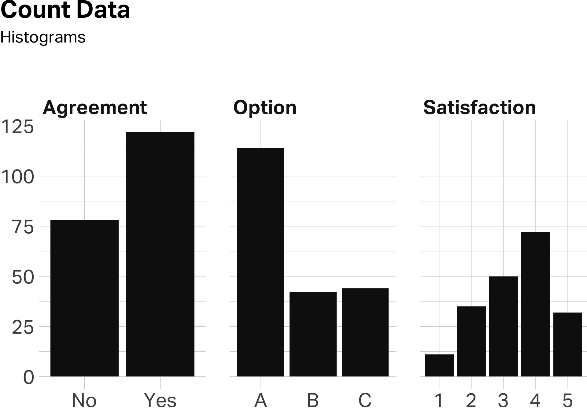
The simplest thing you can do with survey data is count responses. How many people said “yes”? How many chose Option A? How many gave you a 4 or better on satisfaction?
Counts are the raw material. Percentages make them meaningful.
| Variable | score |
|---|---|
| Agreed | 61% |
| Chose A | 57% |
| Satisfied | 52% |
Saying “114 people preferred Brand A” doesn’t tell me much. Saying “57% preferred Brand A” puts it in context.
Means: The Workhorse
The mean is probably the most-used statistic in survey research. Ask people to rate something on a scale, average the responses, report the number. They’re easy to calculate and often easy to interpret. Except when they’re not.
Means work beautifully when responses cluster around a central value. If most people gave you 3s and 4s with a few 2s and 5s sprinkled in, the mean tells a clean story.
But means fall apart when distributions have unusual shapes. Imagine you’ve surveyed 200 customers of a coffee shop, asking them to rate their overall satisfaction on a 1–5 scale. Below are four different distributions of those responses. In each one, the mean is 3.55, but the stories behind each mean are completely different.
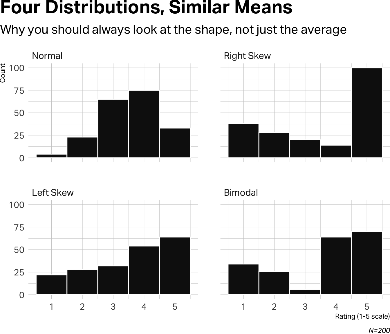
The Normal distribution is the well-behaved case. Responses cluster around the middle, tapering off symmetrically at both ends. The mean of 3.55 accurately represents the typical respondent.
The Right Skew shows responses are affected by a very large distribution of fives (about half of respondents), but without those extreme responses, the distribution indicates an trendline that leans to negative responses.
The Left Skew reflects a largely positive response trend, but there are enough middle and low scores depressing the mean toward the center.
The Bimodal distribution (two peaks instead of one) is the trickiest. You have lovers and haters with almost nobody in the middle. The mean of 3.55 describes a “typical” respondent who doesn’t exist. You don’t have lukewarm customers—you have two distinct groups who feel very differently.
This is why you never report a mean without looking at the distribution first.

Standard Deviation: The Variance Detector
Standard deviation tells you how spread out the responses are. A low SD means people mostly agreed. A high SD means opinions were all over the map. On a 5-point scale, an SD under 1.0 suggests fairly tight agreement; above 1.5 suggests real disagreement
Look at the four distributions we just examined. They all have the same mean (3.55), but their standard deviations tell very different stories:
| Distribution | Mean | SD |
|---|---|---|
| Normal | 3.55 | 0.97 |
| Left Skew | 3.55 | 1.36 |
| Bimodal | 3.55 | 1.50 |
| Right Skew | 3.55 | 1.64 |
The Normal distribution has the lowest SD (0.97)—responses clustered around the center, indicating general agreement. As we move to the skewed and bimodal distributions, SD climbs. The Right Skew has the highest SD (1.64) because responses are polarized between that spike of 5s and everyone else.
When you’re making sense of survey data, start by looking at the distribution. Plot it. But if you’re reporting a mean, always check the standard deviation alongside it. A mean without a measure of spread is only half the story.
Top-Two-Box
Another common way to summarize rating scale data is the “Top-2 Box” (T2B) score—the percentage of respondents who gave a 4 or 5. It’s popular in industry because it’s easy to explain: “67% of customers rated us favorably.”
But look what happens when we apply T2B to our four distributions:
| Distribution | Mean | SD | T2B |
|---|---|---|---|
| Bimodal | 3.55 | 1.50 | 67% |
| Left Skew | 3.55 | 1.36 | 59% |
| Right Skew | 3.55 | 1.64 | 57% |
| Normal | 3.55 | 0.97 | 54% |
Same mean. Very different stories.
The Bimodal distribution—the one with lovers and haters—has the highest T2B score. If you only reported that “67% rated us a 4 or 5,” you’d sound like you’re winning. But you’d be ignoring the 30% who rated you a 1 or 2. That’s not a minor detail.
Meanwhile, the Normal distribution has the lowest T2B, even though it represents the healthiest pattern: broad consensus around the middle with few extremes.
The statistic you choose shapes the story you tell. Means, standard deviations, and Top-2 Box scores each reveal something different—and each can mislead if used in isolation. Good researchers triangulate. They look at the data from multiple angles before drawing conclusions.
III: Cross-Tabulations
At some point, you’ll want to ask, “do different groups respond differently?”
Are women more satisfied than men? Do younger customers prefer the new design? Is there a difference between frequent buyers and occasional ones?
This is where cross-tabulations come in. A cross-tab breaks down your responses by subgroups, so you can compare them side by side.
Remember that Right Skew distribution—the one with the spike of 5s? We wondered: who are those enthusiasts, and why do they feel so differently from everyone else?
Turns out, they’re cold brew buyers.
When we split the satisfaction data by product purchased, the picture sharpens:
| Cold Brew | Other | |
|---|---|---|
| Mean | 4.21 | 3.12 |
| SD | 1.02 | 1.31 |
| T2B | 78% | 44% |
| n | 80 | 120 |
The cold brew customers are devoted—78% rated the shop a 4 or 5, with relatively tight agreement (SD of 1.02). Everyone else? Lukewarm at best. Their mean is a full point lower, and their responses are more scattered.
This is the power of a cross-tab. The overall mean of 3.55 told us almost nothing. But once we segmented by product, we found the story: the cold brew is carrying the business. If that product disappears—or if those customers churn—the numbers collapse.
How to Build a Cross-Tab
Cross-Tabs are simple to build in most applications. Group your data by a categorical variable, then calculate your summary statistics within each group.
In a spreadsheet, you can do this with filters or pivot tables. Filter your data to show only cold brew buyers, calculate the mean. Then filter to show everyone else, calculate again. A pivot table automates this—put your grouping variable (product) in the rows, your outcome variable (satisfaction) in the values, and tell it to compute the average.
We’ll go deeper on cross-tabs later in the course. For now, know two things:
- Cross-tabs are your main tool for finding patterns in survey data.
- Small subgroups lie. If you’re comparing 12 people to 73 people, the smaller group’s numbers will bounce around due to random noise. Don’t over-interpret differences when one group has a tiny sample.
IV: Begin With the End in Mind
Here’s something that will save you grief: before you field a survey, know how you’re going to analyze it.
This sounds obvious. It isn’t. Students routinely build questionnaires, collect responses, and only then ask, “So… what do we do with this?” They end up fishing through the data, trying different cuts, hoping something interesting emerges. This is the research equivalent of throwing spaghetti at the wall and calling whatever sticks “insights.” It’s vibes masquerading as analysis—storytelling untethered from any actual story. Sometimes you stumble onto something interesting. Usually you’re just standing in a river with a fishing rod, wondering why Brad Pitt made this look so cool in A River Runs Through It when you just look cold and wet.

The better approach is to design your study with an analysis plan. Before you write a single question, ask yourself:
- What’s the key metric I need to report? (Mean? Top-two-box? Percentage choosing X?)
- What comparisons matter? (Men vs. women? Heavy users vs. light users? Before vs. after?)
- What would a “good” result look like? What would a “bad” result look like?
If you can answer those questions, you’ll write better survey items—because you’ll know exactly what data you need to produce. You’ll also know, the moment your data comes back, whether you have a story or a shrug.
So … should you report the mean, the median, or the top-two-box?
By now you know the answer: it depends. On what the data looks like. On who you’re communicating to. On what decision the number is supposed to inform.
But if you’ve done this right, you had a hunch about the answer before you ever went to field.